Force Table Lab
Objectives:
The purpose of this lab is to gain experience in working with vector quantities. The lab involves the demonstration of the process of the addition of several vectors to form a resultant vector. Graphical solutions for the addition of vectors will be carried out.
Equipment:
Force table with pulleys, ring and string.
Metric ruler, protractor, graph paper
Experimental Procedure:
We will use an instrument called the Force Table. A ring is placed around a pin in the center of the force table. Strings attached to the ring pull it in different directions. The magnitude (strength) of each pull and its direction can be varied. The magnitude of the string tension (force) is determined by the amount of mass that is hung from the other end of the string. The value of the pull (force) is mg, where g = 9. 81 m/s2 (recall Fw = mg). The force table allows you to demonstrate when the sum of forces acting on the ring equals zero. Under this equilibrium condition, the ring, when released, will remain on the spot.
Experiment with two forces:
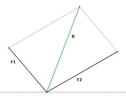
- Place a pulley at the 30o mark on the Force Table and place a total of 0. 35 kg (which includes 0. 05 kg of the mass holder) on the end of the string. Place a second pulley at 130o mark and place a total of 0. 25 kg (including 0. 05 kg of the mass holder). Calculate the magnitude of the forces produced by these masses and record them in Table 1.
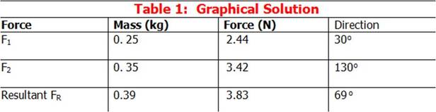
- From the value of the equlibrant force, determine the magnitude and direction of the resultant force and record them in Table 1.
- Find the resultant of these two applied forces by scaled graphical construction using the parallelogram method (See Appendix). Using a ruler and a protractor, construct vectors whose scaled length and direction represent F1 and F2. A convenient scale might be 1 graphical division = 0. 1 N. Read the magnitude and direction of the resultant from your graphical solution and record them in Table 2.
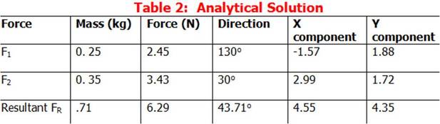
- Using equation 1, calculate the components of F1 and F2 and record them into the analytical solution portion of Table 3. Add the components algebraically and determine the magnitude of the resultant by the Pythagorean Theorem. Determine the angle of the resultant. (See Appendix)
- Calculate the percentage error of the magnitude of the calculated value of FR compared to the graphical analysis solution of FR.
Error Calculation:
Percent error magnitude graphical compared to analytical =
[(Graphical – Analytical)/Analytical] x 100% =
[(3.83-6.29)/6.29] x 100%=39.1%
Discussion:
What sources of error could exist to account for differences between calculated and graphical analysis results?
Percent error magnitude graphical compared to analytical =
[(Graphical – Analytical)/Analytical] x 100% =
[(3.83-6.29)/6.29] x 100%=39.1%
Discussion:
What sources of error could exist to account for differences between calculated and graphical analysis results?
- Error could have occured while graphing due to the lack of percision of the instruments used. Whether one chooses to use a ruler and protractor or a computer program there is a potential for error. Also, human error could have caused us to misread or misuse our instruments. Round-off or arithmetic errors in our calculations could also account for the different results.
